Haystack Node for Information Extraction: A Guide

Transformer-based language models excel at making sense of unstructured textual data, as evidenced by recent results in areas like question answering (QA) and machine translation. But did you know that Transformers can also extract structured information from your textual databases?

Haystack’s EntityExtractor node brings information retrieval to your QA pipelines. It allows you to identify and extract nuggets of structured data, such as named entities or parts of speech, from unstructured text. The possible applications are endless — you could create new metadata, use the extracted information to filter your knowledge base, and enrich or even create entire knowledge graphs.

In this article, we’ll first clarify some terminology around knowledge graphs and information extraction, before diving into a hands-on tutorial on how to use Haystack’s extractor node.

Knowledge Graphs: Uncovering Knowledge through Relationships

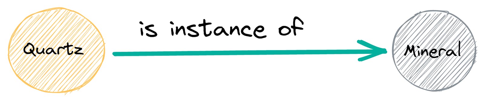
A knowledge graph encodes relationships between entities as a graph-structure that consists of nodes and vertices. These relationships may be conceptualized as relational triples, as in this example: QUARTZ — is_instance_of — MINERAL. Both QUARTZ and MINERAL are entities, while is_instance_of is the vertex that describes their relationship. A great property of knowledge graphs is that they can be easily visualized:

Knowledge graphs are not only used to aggregate established knowledge about the relationships between entities. They can even be instrumental to discovering new information. Combined with machine learning methods, a knowledge graph can help uncover otherwise unknown relationships between entities.

The most famous knowledge graph is probably the one embedded in Google’s search engine. Introduced nearly a decade ago, it uses relationships between entities to create a deeper knowledge representation. Other notable knowledge graphs include Wikidata and DBpedia. Both databases offer structured, easily searchable representations of the mostly unstructured Wikipedia base.

Knowledge graphs can be combined with other datasets to provide new insights, as in the Project Gutenberg Database — which augments and structures the Project Gutenberg text archive with additional metadata from DBPedia.

Introducing the Entity Extractor for Information Extraction

The EntityExtractor is a long-awaited addition to the Haystack framework. It lets you plug in models such as those from the Hugging Face (HF) model hub to extract different kinds of structured information from your documents. The most common use case is Named Entity Recognition (NER). NER models have been pre-trained to extract named entities from text, such as people, locations, and organizations.

An EntityExtractor node can be placed in an indexing or query pipeline. In the first case, the extractor enriches all the documents that are fed to the document store. This process might be slow for large corpora and complex NER models. When the pipeline has finished running, you have at your disposal a database enriched with metadata about persons, locations and other named entities occurring in your text.

As part of a query pipeline, on the other hand, the NER node is placed between the Retriever and the Reader. In this configuration, it only runs on the documents that your extractive QA pipeline has identified during the retrieval process. While much faster than the first method, the downside of this usage is that the metadata is created on the fly and not stored by default.

How to Use the Entity Extractor to Build a Knowledge Graph

To use the EntityExtractor for information extraction, you’ll need to install the latest version of Haystack directly from our repository:

pip install git+https://github.com/deepset-ai/haystack.git
Copied

For our practical example, let’s build a knowledge graph based on a report on mining activities in North Carolina, USA. We want our graph to tell us which resources occur in North Carolina, at which locations, and which companies mine them.

We’ll first build an indexing Pipeline with a node for named entity recognition. It allows us to index the documents automatically with metadata about their named entities. In the second step, we’ll create a query pipeline on top of our indexed documents. We’ll then run a few template questions through the pipeline to retrieve the information we’re interested in, before combining it all in a single knowledge graph in the third and last step.

Step 1: Indexing Pipeline

The text we’ll be using is copied from the website of North Carolina’s Department of Environmental Quality. We stored it in a text file that we named “mining.txt”. To set up our indexing pipeline, we import the following modules:

from haystack.nodes import TextConverter
from haystack.nodes import PreProcessor
from haystack.nodes import EntityExtractor
from haystack.document_stores import ElasticsearchDocumentStore
Copied

We now have to initialize all the nodes before we place them in our pipeline. First comes the TextConverter, which will take care of reading in our text file. We then initialize the PreProcessor, which we instruct to split our document into snippets of 100 words each.

text_converter = TextConverter()
preprocessor = PreProcessor(split_length=100, split_overlap=3, split_respect_sentence_boundary=False)
Copied

Next, we initialize the document store, and just to be on the safe side, we delete any existing documents in there:

document_store = ElasticsearchDocumentStore()
document_store.delete_documents()
Copied

Finally, we set up the entity extractor and pass a BERT-based NER model from HF’s model hub:

entity_extractor = EntityExtractor(model_name_or_path=’dslim/bert-base-NER’)
Copied

We can now construct the pipeline with the initialized components. We place the entity extractor after the preprocessor, to make sure the recognized named entities are aligned with the new structure of our documents:

index_pipe = Pipeline()
index_pipe.add_node(text_converter, ‘TextConverter’, [‘File’])
index_pipe.add_node(preprocessor, ‘PreProcessor’, [‘TextConverter’])
index_pipe.add_node(entity_extractor, ‘EntityExtractor’, [‘PreProcessor’])
index_pipe.add_node(document_store, ‘DocumentStore’, [‘EntityExtractor’])
Copied

We run our text file through the pipeline. Note that the pipeline expects a list as its input:

index_pipe.run(['mining.txt’])
Copied

With a single run() command, we read in our document, split it into shorter text passages, perform information extraction in the form of named entity recognition, and index the enriched documents into our database. We can then extract the documents along with their metadata:

documents = document_store.get_all_documents()
Copied

Let’s take a closer look at one of the documents in our database:

documents[1]

>>> {‘content’: ‘nation in the production of clay used for brick manufacture and ranks seconds in phosphate rock production. North Carolina does not produce significant quantities of metallic minerals but has potential resources.\n\nIndustrial minerals are mined thoughout North Carolina in the Mountain, Piedmont and Coastal Plain provinces.’, ‘content_type’: ‘text’,
‘score’: None,
‘meta’: {‘_split_id’: 1,
  ‘entities’: [
    {‘entity_group’: ‘LOC’, ‘score’: 0.9991990923881531,‘word’: ‘North Carolina’, ‘start’: 108, ‘end’: 122},
    {‘entity_group’: ‘LOC’, ‘score’: 0.957325279712677, ‘word’: ‘Mountain’, ‘start’: 276, ‘end’: 284},
    {‘entity_group’: ‘LOC’, ‘score’: 0.991599440574646, ‘word’: ‘Piedmont’, ‘start’: 286, ‘end’: 294},
    {‘entity_group’: ‘LOC’, ‘score’: 0.9927359819412231, ‘word’: ‘Coastal Plain’, ‘start’: 299, ‘end’: 312}]},
‘embedding’: None,
‘id’: ‘ce52afa9c264f03f28583de8044361c6’}
Copied

The extracted list of entities contains not only information about the type and location (‘start’ and ‘end’) of each named entity, but also the confidence (‘score’) with which the model recognized it. We will use that property to create lists of the organizations and locations mentioned throughout the corpus. Let’s first extract all the entities:

entities = [doc.meta[‘entities’] for doc in documents]
Copied

The result is a nested list, which we’ll want to flatten before we proceed:

flat_entities = [ent for ent_list in entities for ent in ent_list]
Copied

From this list, we can now extract all locations and organizations, using the score as a filter. We only want to keep the entities that were recognized with a confidence of 99 percent or greater.

locations = [ent[‘word’] for ent in flat_entities if ent[‘entity_group’] == ‘LOC’ and ent[‘score’] > .99]
Copied

We’ll do the same for organizations:

organizations = [ent[‘word’] for ent in flat_entities if ent[‘entity_group’] == ‘ORG’ and ent[‘score’] > .99]
Copied

Let’s have a look at all the organizations in our dataset. We turn them into a set to avoid printing out duplicates:

set(organizations)

>>> {‘North Carolina Phosphate Corporation’, ‘NCGS’, ‘##gates Company’, ‘Potash Corporation of Saskatchewan’, ‘Wake Stone Corporation’, ‘RGC’, ‘Marine Uranium Corporation’, ‘North Carolina Granite Company’, ‘Vulcan Materials Company’, ‘Mobil Oil Corporation’, ‘Martin Marietta A’, ‘NCPC’, ‘Nello L. Teer Company’, ‘Jacobs Creek Stone Company’, ‘Texasgulf, Incorporated’}
Copied

If you look closely, you’ll see that one of the names does not seem right: ‘##agates Company’ does not look like a legitimate company name. That’s because it’s really part of the name ‘Martin Marietta Aggregates Company.’ BERT uses the clever WordPiece algorithm to split unknown words into sub-word units. We’ll see later how these split entities can be easily recombined in Haystack.

Step 2: Query Pipeline

Let’s now build the second pipeline needed to perform information extraction on our documents. We’ll be importing the retriever, reader, and pipeline modules:

from haystack.nodes import DensePassageRetriever
from haystack.nodes import FARMReader
from haystack.pipelines import ExtractiveQAPipeline
Copied

Let’s initialize the dense passage retriever and use it to update the documents in our database with dense text vectors:

retriever = DensePassageRetriever(document_store=document_store)
document_store.update_embeddings(retriever)
Copied

Next, we initialize the reader with a pre-trained RoBERTa model and combine both reader and retriever in an extractive QA pipeline:

reader = FARMReader(model_name_or_path=”deepset/roberta-base-squad2")

query_pipe = ExtractiveQAPipeline(reader=reader, retriever=retriever)
Copied

We now create a list of natural resources that we want to ask questions about:

resources = [‘clay’, ‘dimension stone’, ‘sand’, ‘mica’, ‘olivine’, ‘phosphate’, ‘pyrophillite’, ‘coal’]
Copied

For each resource, we’re interested in two questions: ”where does the resource occur?” and “which company mines it?” We create two answer dictionaries, one for the places of occurrence and one for the mining companies:

occurrences = {}
companies = {}
Copied

We then run a for-loop on our list of resources that runs both our questions through the system:

for resource in resources:
  occurrence = query_pipe.run(query=f’Where does {resource} occur?’, params={‘Reader’: {‘top_k’: 3}})
  occurrences[resource] = occurrence
  company = query_pipe.run(query=f’Which company mines {resource}?’, params={‘Reader’: {‘top_k’: 3}})
  companies[resource] = company
Copied

Step 3: Making Sense of the Extracted Entities

We’ve instructed our reader to return three results per resource and question. But not all of these results will be useful. The simplify_ner_for_qa() function extracts the named entities that really occur in the returned answer. It also takes care of joining together the sub-word units that we saw earlier. Let’s apply it to all of the answers in our dictionaries:

from haystack.nodes.extractor import simplify_ner_for_qa

occurrences_simplified = {k: simplify_ner_for_qa(v) for k, v in occurrences.items()}
companies_simplified = {k: simplify_ner_for_qa(v) for k, v in companies.items()}
Copied

Let’s have a look at the simplified results for companies that mine phosphate:

companies_simplified[‘phosphate’]

>>> [{‘answer’: ‘Potash Corporation of Saskatchewan’, ‘entities’: [‘Potash Corporation of Saskatchewan’]}, {‘answer’: ‘North Carolina Phosphate Corporation’, ‘entities’: [‘North Carolina Phosphate Corporation’]}, {‘answer’: ‘Beaufort County’, ‘entities’: [‘Beaufort County’]}]
Copied

All results are named entities — but some of them designate locations rather than companies, a difference that our reader model failed to pick up on. Let’s apply another filter to make sure we only have the right kind of named entity in our answer dictionaries. To that end, we’ll use the sets of organizations and locations that we extracted from our knowledge base earlier:

companies_verified = {k: [ans[‘answer’] for ans in v if ans[‘answer’] in organizations] for k, v in companies_simplified.items()}
Copied

Here is the final results dictionary for the companies:

companies_verified

>>> {‘clay’: [‘Nello L. Teer Company’], ‘dimension stone’: [‘Jacobs Creek Stone Company’], ‘sand’: [‘Nello L. Teer Company’], ‘mica’: [‘Southeast Tisand’], ‘olivine’: [‘Texasgulf, Incorporated’], ‘phosphate’: [‘Potash Corporation of Saskatchewan’, ‘North Carolina Phosphate Corporation’], ‘pyrophillite’: [‘Potash Corporation of Saskatchewan’, ‘Texasgulf, Incorporated’], ‘coal’: []}
Copied

Let’s do the same for the occurrences dictionary. Only the answers that are present in our locations set will be verified:

occurrences_verified = {k: [ans[‘answer’] for ans in v if ans[‘answer’] in locations] for k, v in occurrences_simplified.items()}
Copied

And the final occurrences dictionary:

occurrences_verified

>>> {‘clay’: [‘Murphy’], ‘dimension stone’: [], ‘sand’: [], ‘mica’: [], ‘olivine’: [‘Blue Ridge’, ‘North Carolina’], ‘phosphate’: [‘Beaufort County’], ‘pyrophillite’: [‘Beaufort County’], ‘coal’: [‘Deep River Triassic Basin’]}
Copied

We can now use the information encoded in the two answer dictionaries to create a knowledge graph using a graph database like Neo4j or a framework like Apache Jena. The final graph might end up looking like the following:

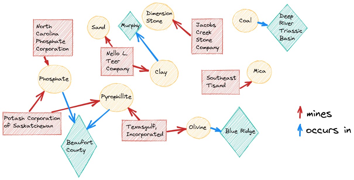
The graph neatly captures some of the relationships in our text. For example, we now know that the Potash Corporation of Saskatchewan mines both potassium and pyrophyllite, and we also understand why: Both resources occur in Beaufort County. We could even try to use some of the information from the graph to speculate on or infer new relationships.

Our graph captures the occurrence of clay in Murphy; however, it doesn’t say where sand can be found. Based on the fact that both resources are mined by the same company (Nello L. Teer), we might speculate that sand occurs in Murphy as well. Recall that our graph is non-exhaustive — for one, we only captured high-confidence locations and companies — so we cannot draw the inference. But our exercise demonstrates how a knowledge graph might be used to unearth new information.

In the case of our document — which is reasonably short — we could have extracted the entities and their relationships by doing a close reading of the text. But imagine you wanted to perform information extraction on a much larger textual knowledge base. Thanks to Haystack, we could easily scale the methods outlined in this article to collections that span tens of thousands of texts. By running them first through the indexing and then the query pipeline, we would be able to create a structured knowledge graph to provide us with in-depth information about the corpus’ entities and their connections at one glance.

Start Mining Your Texts with Haystack

The EntityExtractor is still in its infancy and will likely undergo a few changes in the upcoming months. But we wanted to share our excitement about this new node with you as early on as possible, and show you how you can use it to unearth valuable information that will enrich your knowledge bases.

We invite you to head over to our GitHub repository and be one of the first to apply the new node to your use cases. And if you like what you see, make sure to leave us a star :)